Variational Autoencoders from Scratch
| GitHub Repo 👾 | Scope: ⭐⭐⭐ |
Learning is compression
One of the first things one can do with a neural network is to create an autoencoder, or AE. An autoencoder is a neural network that is trained to predict its input, but is structured so that the network “funnels” information through a smaller space before being expanded out. This smaller space is often called the latent space, and the task of predicting input is often called reconstruction.
The portion of the network that maps the input to the latent space is called the encoder, and the part that maps the latent space to the prediction is the decoder.
If we denote $x$ as the input and $x’$ as the reconstruction, an autoencoder might use the sum of squared errors loss function to train on, like so.
\[\mathcal{L} = \frac{1}{2}\sum_{i}(x_i - x_i')^2\]Writing and training an AE after my neural network was little more than writing a wrapper around the network class to add an encode and decode method. However, even though I was able to achieve a strong reconstruction of the data, slight perturbations to the latent space led to poor reconstructions. This is because as the vanilla AE loss solely prioritizes the task of reconstruction, the latent space is often unorganized. This means that points in the latent space that aren’t derived directly from data often decode into a blurry mess.
This is bad if one wants not just to compress the data, but generate plausible samples from the original data distribution.
Structure that representation!
It turns out there is a way to train a network that also prioritizes latent space organization! These networks are called variational autoencoders, or VAEs for short. After I watched this excellent YouTube video by Deepia, VAEs became the next network architecture I chose to implement from scratch.
A VAE, like a vanilla AE, consist of an encoder neural net $E$ and decoder neural net $D$. However, the forward pass of the network predicts the parameters of a (multivariate) normal distribution, namely $\mu$ and $\log(\sigma)$.
\[E(x) = (\mu, \log(\sigma))\]We predict $\log(\sigma)$ instead of $\sigma$ so that the training process doesn’t create $0$ deviation distributions.
Then the input $z$ to the decoder net is a sample from this predicted distribution. The key idea for VAEs is not just that the encoder learns to map data to a distribution (and not a single point as AEs do), but also how to make this sampling process differentiable. Sampling from this distribution is done using the reparapetrization trick, which for our case is just writing $z$ as follows
\[z = \mu + \epsilon \exp(\log \sigma),\]where $\epsilon$ is a sample from the (multivariate) standard normal.
As for the training of such a network, the loss function for VAEs has two components. We have the usual reconstruction loss, written \(\mathcal{L}_{rec}\) , and the regularization loss, written $\mathcal{L}_{reg}$. The regularization loss is a mathematical expression for how far away the distribution created by the encoder, called $P$ differs from some given distribution, called $Q$. VAEs choose this $Q$ to be the (multivariate) standard normal distribution. This means that as we train the learning process also prioritizes moving our encoded data into the more “organized” normal distribution.
More specifically, the regularization loss is the Kullback-Leibler divergence between the created normal distribution to the standard normal. KL divergence is usually complicated to compute, but the divergence between two Gaussians can be symbolically written. This gives the full loss function for VAEs as
\[\mathcal{L} = \mathcal{L}_{rec} + \mathcal{L}_{reg} = \frac{1}{2}\sum_{i}(x_i - x_i')^2 - \frac{1}{2}\sum_{i}(1+2\log(\sigma_i)-\mu_i^2-\sigma_i^2).\]Because I have yet to implement an automatic differentiation engine, and I couldn’t find anything on the internet, I had to compute the gradients for a VAE by hand. I first rewrote the regularization portion of the loss to match the output of $E$, namely
\[\mathcal{L}_{reg} = \frac{1}{2}\exp(2\log\sigma) + \frac{1}{2}\mu^2 - \log\sigma - \frac{1}{2}.\]Then we can compute the gradient $\frac{\partial \mathcal{L}}{\partial z}$ efficiently after a forward pass of the full network with the following equations.
\[\begin{eqnarray*} \frac{\partial \mathcal{L}_{rec}}{\partial \log{\sigma}} & = & \frac{\partial \mathcal{L}_{rec}}{\partial z}\frac{\partial z}{\partial \log{\sigma}} = \frac{\partial \mathcal{L}_{rec}}{\partial z} \epsilon \exp(\log\sigma) \\ \frac{\partial \mathcal{L}_{rec}}{\partial \log{\sigma}} & = & \frac{\partial \mathcal{L}_{rec}}{\partial z}\frac{\partial z}{\partial \log{\sigma}} = \frac{\partial \mathcal{L}_{rec}}{\partial z} \epsilon \exp(\log\sigma) \\ \frac{\partial \mathcal{L}_{reg}}{\partial \mu} & = & \mu \\ \frac{\partial \mathcal{L}_{reg}}{\partial \log{\sigma}} & = & \exp(2\log \sigma) - \vec{1} \end{eqnarray*}\]I also had to come up with a clever way to write a VAE given how I chose to implement the neural network class from the previous project, where I had to write a second loss function that only referenced $\cal{L}_{reg}$ in the middle of the network. However, the learning turned out to be extremely slow, and bottomed out on an overall bad performance (predicting the average $x$ instead of returning a similar image to $x$). I determined that this was because I was only using my implementation of vanilla stochastic gradient descent. SGD was not performing well because the gradient was “doubly-stochastic”, in the sense that randomness in the gradient vector was introduced both from the minibatching (as usual) and from the inserted noise $\epsilon$. The gradients were too noisy to learn much.
Wait, momentum is crucial? …always has been
To fix this I read through the famous Adam Optimizer paper, which is a nearly ubiquitous optimizer in modern ML work. This is another Diedrik Kingma invention that has proved its staying power.
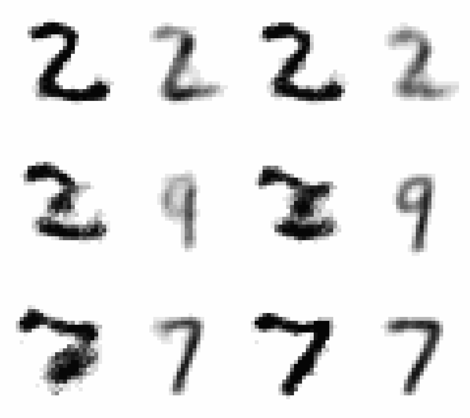
After implementing this I saw a staggering improvement in learning (~10x decrease in the scale of the loss compared to using SGD), showing the clear power of momentum-based optimization. After training, I wanted to produce an animation comparing AEs and VAEs when extrapolating in the latent space. This animation shows the decoded transitions between a latent representation for a 2 and a 7.
Notice that as the AE only prioritizes reconstruction, the image is much sharper than that of the VAE. However, the VAE’s transition between the two is smoother, and more often looks like some type of digit in the transition. We can see the 2 go to a 9 and then to a 7 smoothly.
As VAEs served as the beginning of the generative AI boom, I set my sights next on diffusion models, the current state of the art for image generation. I explore these models in a future post!
Thanks for reading!

