[MLCS] Neural Networks from Scratch
| NN GitHub Repo 👾 | RL GitHub Repo 👾 | Scope: ⭐⭐⭐⭐ |
Wow Machine Learning is Cool
Even before I studied the subject, I found machine learning fascinating. To me it was some confusing, amorphous new technique blazing past traditional programming. I remember my feeling of true amazement hearing the results of a chess match between two computer programs, AlphaZero vs Stockfish. Stockfish was the long-time champion, being coded with the help of Grandmaster chess players. AlphaZero was the challenger, only playing chess against itself for four hours. AlphaZero’s performance improved over those four hours using techniques from deep reinforcement learning, a topic so dense I thought I had no hope of ever understanding it.
AlphaZero’s crushing victory marked a similar paradigm shift in the world of chess to the Kasparov vs DeepBlue match some two decades prior. The prior shift was that now software could beat the “learned software” of the human brain in a complicated competetive domain. With the AlphaZero vs Stockfish match, we saw our ability to write software being surpassed. Our understanding of what even makes a good chess move was now second to what the machine “thought”. And even worse, it surpassed the collective understanding of our hundreds of years of experience in four hours. I knew I had to learn how these programs worked. But how?
Machine Learning’s Pedagogy Problem
I was lucky enough to accidentally study all the prerequisites for machine learning before I even started. The math was not a haze on my understanding, but instead my strength. In fact, I was happy to dive into the computation! But when I finally felt I was able to study the subject, I faced a major disappointment. I took multiple courses, and yet none would explain how the learning was actually happening!
Each time I would work through a Jupyter notebook, I would inevitabely get to a line that looked like this:
    ...
    model.train()
    ...
I would almost scream “What is .train() doing!?” The thing I wanted from the course most was reduced to a single line. Worst of all, my instructors often downplayed the details as “laborious” and “uninteresting applications of the chain rule”. Well they weren’t uninteresting to me!
To clarify, I understand that hiding complexity is what programming is all about. It is necessary for ease of use, and I use frameworks like sklearn and PyTorch all the time. But my intellectual curiosity felt like it was slamming into a brick wall. So I decided I would have to go out on my own. I was going to do it from scratch.
Neural Networks from Scratch
My interest in deep learning led me to the excellent textbook Neural Networks and Deep Learning by Michael Nielsen. I follow the notation laid out in this text, namely that a feed forward neural network is defined for layers $2 \leq \ell \leq L$ as
\[z^{\ell} = w^{\ell}a^{\ell-1} + b^{\ell}\] \[a^{\ell} = \sigma^{\ell}(z^{\ell})\]for activation functions $\sigma^{\ell}$, weights $w^{\ell}$ and biases $b^{\ell}$. Note that the weights and biases are almost always matrices.
NOTE: Superscripts are layer indexes and not exponentiation, unless otherwise stated.
Above is a replication of a diagram from Nielsen’s textbook detailing how his notation describes a “ball and stick” diagram of a neural network. The red “stick” denotes the weight $w^3_{2,4}$. This is the notation I use throughout the project and this post.
Even this textbook lists the backpropagation chapter as optional reading, but the chapter was beautifully written all the same. After reading through it in its entirety, intentionally avoiding the provided implementations, I returned to the backpropagation chapter. Nielsen defines the algorithm as follows. Define the error $\delta_j^{\ell}$ of neuron $j$ at layer $\ell$ be
\[\delta_j^{\ell} = \frac{\partial C}{\partial z_j^\ell}\]Then backpropagating the error can be conducted using the following equations
\[\begin{eqnarray*} \delta^L & = & \nabla_a C \cdot \sigma'^{L}(z^L) \\ \delta^{\ell} & = & ((w^{\ell+1})^{T}\delta^{\ell+1}) \cdot \sigma'^{\ell}(z^{\ell}) \\ \frac{\partial C}{\partial b_j^\ell} & = & \delta_j^{\ell} \\ \frac{\partial C}{\partial w_{jk}^\ell} & = & a_k^{\ell-1}\delta_j^{\ell} \end{eqnarray*}\]For a while I struggled with the intuition as to why the error would be defined as a gradient. Though Nielsen describes this well, it just seemed too perfect, and consequently took a long time to “sit right” with me.
But after doing my own derivations for a small network, I felt as if I really could write a neural network from scratch. And that is what I did. After a series of stressful nights, I did complete the project. I encountered a series of difficult bugs, including after my network was running but failing to learn. The bug that took longest to find was an erroneous summation of the weight gradients in a batch, as opposed to an average. But after I weeded all these issues out, I’m happy to say I completed the project. Below is an interactive demo for MNIST using a network written and trained entirely from scratch.
TODO demo, credit
This level of understanding not only grounded my understanding of the topic, but it also further motivated my study of deep learning. Now that I had a neural network from scratch, what else could I do?
(Variational) AutoEncoders from Scratch
One of the first things one can do with a neural network is to create an autoencoder. An autoencoder is a neural network that is trained to predict its input, but is structured so that the network “funnels” information through a smaller space before being expanded out. This smaller space is often called the latent space, and the task of predicting input is often called reconstruction.
The portion of the network that maps the input to the latent space is called the encoder, and the part that maps the latent space to the prediction is the decoder.
If we denote $x$ as the input and $x’$ as the reconstruction, an autoencoder might use the sum of squared errors loss function to train on, like so.
\[\mathcal{L} = \frac{1}{2}\sum_{i}(x_i - x_i')^2\]Writing and training an AE after my neural network was little more than writing a wrapper around the network class to add an encode and decode method. However, even though I was able to achieve a strong reconstruction of the data, slight perturbations to the latent space led to poor reconstructions. This is because as the vanilla AE loss solely prioritizes the task of reconstruction, the latent space is often unorganized. This means that points in the latent space that aren’t derived directly from data often decode into a blurry mess.
This is bad if one wants not just to compress the data, but generate plausible samples from the original data distribution. It turns out there is a way to train a network that also prioritizes latent space organization! These networks are called variational autoencoders, or VAEs for short. After I watched this excellent YouTube video by Deepia, VAEs became the next network architecture I chose to implement from scratch.
A VAE, like a vanilla AE, consist of an encoder neural net $E$ and decoder neural net $D$. However, the forward pass of the network predicts the parameters of a (multivariate) normal distribution, namely $\mu$ and $\log(\sigma)$.
\[E(x) = (\mu, \log(\sigma))\]We predict $\log(\sigma)$ instead of $\sigma$ so that the training process doesn’t create $0$ deviation distributions.
Then the input $z$ to the decoder net is a sample from this predicted distribution. The key idea for VAEs is not just that the encoder learns to map data to a distribution (and not a single point as AEs do), but also how to make this sampling process differentiable. Sampling from this distribution is done using the reparapetrization trick, which for our case is just writing $z$ as follows
\[z = \mu + \epsilon \exp(\log \sigma),\]where $\epsilon$ is a sample from the (multivariate) standard normal.
As for the training of such a network, the loss function for VAEs has two components. We have the usual reconstruction loss, written \(\mathcal{L}_{rec}\) , and the regularization loss, written $\mathcal{L}_{reg}$. The regularization loss is a mathematical expression for how far away the distribution created by the encoder, called $P$ differs from some given distribution, called $Q$. VAEs choose this $Q$ to be the (multivariate) standard normal distribution. This means that as we train the learning process also prioritizes moving our encoded data into the more “organized” normal distribution.
More specifically, the regularization loss is the Kullback-Leibler divergence between the created normal distribution to the standard normal. KL divergence is usually complicated to compute, but the divergence between two Gaussians can be symbollically written. This gives the full loss function for VAEs as
\[\mathcal{L} = \mathcal{L}_{rec} + \mathcal{L}_{reg} = \frac{1}{2}\sum_{i}(x_i - x_i')^2 - \frac{1}{2}\sum_{i}(1+2\log(\sigma_i)-\mu_i^2-\sigma_i^2).\]Because I have yet to implement an automatic differentiation engine, and I couldn’t find anything on the internet, I had to compute the gradients for a VAE by hand. I first rewrote the regularization portion of the loss to match the output of $E$, namely
\[\mathcal{L}_{reg} = \frac{1}{2}\exp(2\log\sigma) + \frac{1}{2}\mu^2 - \log\sigma - \frac{1}{2}.\]Then we can compute the gradient $\frac{\partial \mathcal{L}}{\partial z}$ efficiently after a forward pass of the full network with the following equations.
\[\begin{eqnarray*} \frac{\partial \mathcal{L}_{rec}}{\partial \log{\sigma}} & = & \frac{\partial \mathcal{L}_{rec}}{\partial z}\frac{\partial z}{\partial \log{\sigma}} = \frac{\partial \mathcal{L}_{rec}}{\partial z} \epsilon \exp(\log\sigma) \\ \frac{\partial \mathcal{L}_{rec}}{\partial \log{\sigma}} & = & \frac{\partial \mathcal{L}_{rec}}{\partial z}\frac{\partial z}{\partial \log{\sigma}} = \frac{\partial \mathcal{L}_{rec}}{\partial z} \epsilon \exp(\log\sigma) \\ \frac{\partial \mathcal{L}_{reg}}{\partial \mu} & = & \mu \\ \frac{\partial \mathcal{L}_{reg}}{\partial \log{\sigma}} & = & \exp(2\log \sigma) - \vec{1} \end{eqnarray*}\]I also had to come up with a clever way to write a VAE given how I chose to implement the neural network class from the previous project, where I had to write a second loss function that only referenced $\cal{L}_{reg}$ in the middle of the network. However, the learning turned out to be extremely slow, and bottomed out on an overall bad performance (predicting the average $x$ instead of returning a similar image to $x$). I determined that this was because I was only using the vanilla stochastic gradient descent. SGD was not performing well because the gradient was “doubly-stochastic”, in the sense that randomness in the gradient vector was introduced both from the minibatching (as usual) and from the inserted noise $\epsilon$. This lead to noisy learning.
To fix this I read through the famous Adam Optimizer paper, which is a nearly ubiquitous optimizer in modern ML work. After implementing this I saw a staggering improvement in learning (~10x decrease in the scale of the loss compared to using SGD), showing me the clear power of momentum-based optimization.
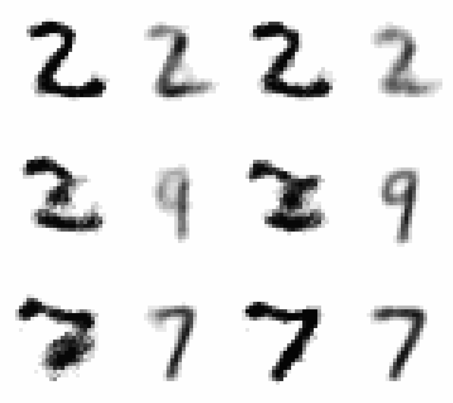
After training, I wanted to produce an animation comparing AEs and VAEs when extrapolating in the latent space. This animation shows the decoded transitions between a latent representation for a 2 and a 7.

Notice that as the AE only prioritizes reconstruction the image is much sharper than that of the VAE. However, the VAE’s transition between the two is smoother, and more often looks like some type of digit in the transition.
As VAEs served as the beginning of the generative AI boom, I set my sights next on diffusion models, the current state of the art for image generation.
Diffusion from Scratch
Diffusion models, popularized in the famous paper Denoising Diffusion Probabilistic Models, are the current state of the art for image generation.
Implementing one from scratch proved difficult, especially for the limited tools I had at my disposal (that I had implemented from scratch). I had to make a proper diffusion model with no convolution layers (or skip connectios for UNET-like architectures) and no GPU-enabled training because I have not learned CuPy yet. In hindsight, I went into this project underprepared, but I was still able to walk away with something cool to show.
I chose to train my network on the EMNIST dataset (as opposed to the MNIST dataset) for more striking final generation. I initially tried to train a diffusion model with the base neural network class I had written before on the raw pixels. This proved to be unfeasible. I’m not sure why the performance using a base neural network was so poor. It’s likely that when I sit down to write convolutional layers from scratch, that I will be able to get better performance conducting diffusion on raw pixels.
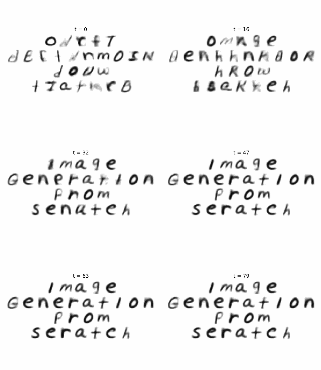
At the time, however, I decided that my best option was to use my previously implemented VAE to reduce the dimensionality of the input, and then conduct diffusion on the latent representation. This means that I technichally implemented a LDDPM as opposed to a vanilla DDPM model. This allowed for much better conditional image generation to be learned just on my CPU. I also wrote some code to structure the generations into short sentences, shown below.

As you can see, the blurring artifacts from the VAE decoder are present in the final animation, and some of the generation lacks variety (such as the letter ‘I’). Regardless, the noising and sampling process was a fun thing to learn, and I was very proud of the final result. I had a lot of fun sending messages to my friends with the final trained network.
With my neural architectures completed for now, I wanted to focus on the third type of learning – the algorithms that originally got me into ML – reinforcement learning.
Reinforcement Learning from Scratch
As RL was the subject I had been thinking about the longest, it was the subject I had the best idea for a project with. I had been playing 2048 since it was released, and I always knew it was a perfect choice for a beginner reinforcement learning project. It has a large state space, small action space, non-trivial strategies, and a clearly defined reward function. The game is also entirely open source, which was a real bonus.
I decided I would make the bot after I completed the Sutton and Barto textbook. It was an intense summer read, and by the time I completed it I was itching to get started. The first challenge the project posed was the game itself. I initially used a pre-built Python implementation called Macht, but later chose to implement the game from scratch to speed up training as much as possible.
As for the learning algorithm, I initially wanted to do policy optimization, as opposed to TD or Q learning. I really liked the idea of having a single neural network that just takes in a board state and plays a good move. However, the performance was really poor (I learned later that the reason training went poorly was that I didn’t implement a replay buffer of past games, and was just training the network on a single board, reward pair. This was so noisy that the network failed to learn anything). I abandoned the technique quickly, and the (self-imposed) setback led me to see if other people had written 2048 RL bots.
I was surprised to find that not only have people written 2048 RL bots, but there is serious academic research on the subject. I looked at a series of papers, the most important being Temporal Difference Learning of N-Tuple Networks for the Game 2048 by Szubert and colleagues. They showed that TD learning with a RAMnet approximator worked well, and so I chose to pursue this.
There was a gruelling episode of debugging this implementation. Like the many other RL-from-scratch projects I had read about, the “code runs but learning fails” part of the ML development pipeline was arduous.
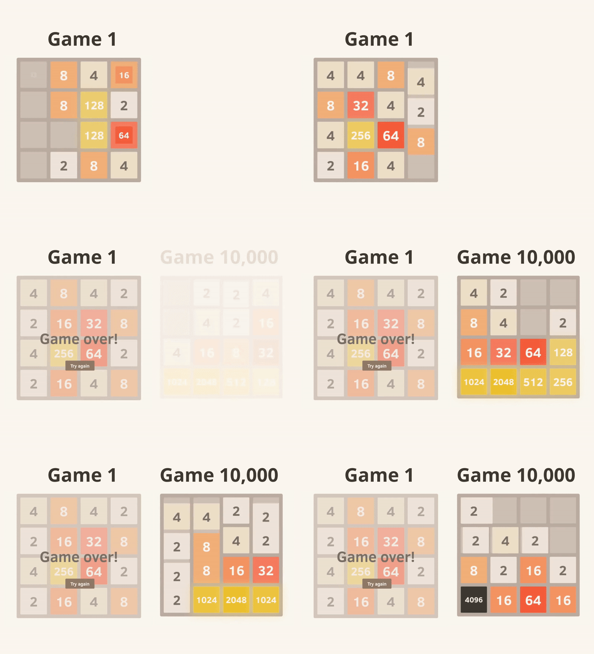
It is hard to describe the feeling of elation of finally seeing my algorithm learning to play one of my favorite games. After training for ~10,000 games, the agent achieves the 2048 tile 49.1% of the time, and achieves the 4196 tile 1.5% of the time.
Now that the bot was trained, the final step was hooking up the history of the game to play on the real game’s visualizer. I cloned the original repo and changed the internal Javascript to play a JSON history to make the final animation. I decided to showcase one of my agent’s best games, shown below.

This was one of my favorite animations to create, and I still enjoy watching it to this day.
Future Work
Before I complete my graduate studies, I really hope to implement both a CNN and a Transformer from scratch. This would complete from-scratch implementations for what I would call the main suite of machine learning models. I look forward to writing future posts about these projects!
Thanks for reading!