Parameter Golfing Tic Tac Toe
"The only winning move is not to play" - WOPR
| GitHub Repo 👾 | Scope: ⭐⭐⭐ |
I clearly have a thing for making useless equations for games. This time, I have turned my attention to tic tac toe. I wanted to know: How small of an equation can perfectly play the game?
The Problem
The first thing I should point out is that tic tac toe is classically solved by the minimax algorithm, which is a simple algorithm that runs for tic tac toe in a fraction of a second on a modern computer. My goal is different though: I want a way a human could play the game perfectly.
It turns out that there technically does exist a relatively small algorithm in natural language, for playing optimal tic tac toe, which can be found on the game’s Wikipedia page. The algorithm, owed to Newell and Simon, is to pick the first available move that matches the criterion from the following list:
Newell and Simon’s Strategy
- Win: If the player has two in a row, they can place a third to get three in a row.
- Block: If the opponent has two in a row, the player must play the third themselves to block the opponent.
- Fork: Cause a scenario where the player has two ways to win (two non-blocked lines of 2).
- Blocking an opponent’s fork: If there is only one possible fork for the opponent, the player should block it. Otherwise, the player should block all forks in any way that simultaneously allows them to make two in a row. Otherwise, the player should make a two in a row to force the opponent into defending, as long as it does not result in them producing a fork. For example, if “X” has two opposite corners and “O” has the center, “O” must not play a corner move to win. (Playing a corner move in this scenario produces a fork for “X” to win.)
- Center: A player marks the center. (If it is the first move of the game, playing a corner move gives the second player more opportunities to make a mistake and may therefore be the better choice; however, it makes no difference between perfect players.)
- Opposite corner: If the opponent is in the corner, the player plays the opposite corner.
- Empty corner: The player plays in a corner square.
- Empty side: The player plays in a middle square on any of the four sides.
This strategy may be useful to some players, but steps 3 and 4 seem hard to follow for me. I want to improve this list by reducing steps 3-8 into something that a person could memorize to become a perfect tic tac toe player.
For other requirements and design choices, I also wanted my equation to be a strong solution to the game as opposed to a weak solution, which means that algorithm would be optimal no matter what (legal & reachable) position it was given.
Another design choice requires a discussion on the data we hope to support.
The Data
Though minimax isn’t a solution to our problem, it can certainly find the optimal moves for each position! Looping over all possible position yields 4520 total board positions, and the moves that are optimal at each of these positions. Critically, for many positions there are multiple moves that result in the same outcome. For example, in the following position ‘X’ can win in three different ways.
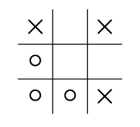
So which one should I choose my equation to play? I wanted a simple solution above all else, which means that I won’t, say, choose moves by some other heuristic (like how many opportunities a move gives for the opponent to make a mistake, etc.). I will instead choose what move is picked by whatever works to make as simple as possible an equation.
Another design choice is how I should represent the board. In line with my simple algorithm approach, I needed a simple, easy to follow way to encode the board into numerical entries.
The Representation. The board is represented by 9 numbers that are either 0, 1, or -1. We represent ‘X’s with 1, ‘O’ with -1, and 0 for blank spaces, reading position top-to-bottom, left to right.
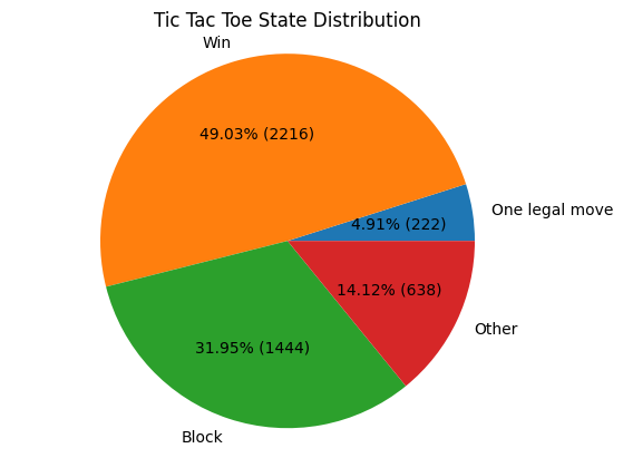
Furthermore, there are plenty of data points that the equation does not need to handle. As the main goal of this equation will be to help human players, we can discard a large portion of the 4520 tic tac toe positions. We leave positions to the human in which there is one legal move (222 positions), moves where the game can be won in one move (2216 positions), and moves that immediately block an opponent from winning (1444 positions). This leaves 638 positions to the equation to model properly.
The Zoo of Solutions
I considered a myriad of possible solutions to this problem. Decision trees? Too much to memorize. Treating the whole problem as circuit minimization and using the espresso minimizer? Ran, but result was too much to memorize. Symbolic regression? Never converged. Evolutionary computation? Also never converged.
As a machine learning researcher, the idea of using a neural network whispers in your ear like the green goblin mask. Though neural networks are also hard to memorize, and for this sort of project a pretty lame solution, I decided to explore the possibility. Out the gate, I decided to get small and simple, the architecture would be a simple single-hidden unit network with ReLU activations. As the board has 9 squares, the input and output dimensions would be 9. Other than this standard setup, there are three interesting things about training a tiny neural network on this dataset.
The first is only slightly interesting. We can do illegal move masking to remove the constraint on portions of the network dedicated simply to downweighting illegal moves. This is achived just by applying the masking in the forward pass, namely:
1
2
3
4
5
6
def forward(self, x):
  y = self.model(x)
  # mask moves that have already been made, ie. elements in the representation that are nonzero
  illegal = (x != 0)
  y = y.masked_fill(illegal, mask_val)
  return y
The seconds is that this dataset has many data points in which there are multiple correct labels. A neural network that has a final output layer as an argmax can only choose one move for each data point, and so the question is which one? There are way too many choices to just train one neural network per configuration, and picking randomly may be non optimal for the goal to make the smallest possible network. Instead, I decided that the label itself would change over the course of training, such that it was the legal optimal move with largest logit at the time of each forward pass. That looked like this, where moves_mask was a boolean tensor that was shape (num_positions, 9) possible moves, and True if the move at that position was optimal, and False else.
1
2
3
4
5
6
7
8
9
outputs = model(data_tensor)

# NOTE the ground truth is the legal optimal move with largest logit
masked_outputs = outputs.masked_fill(~(moves_mask.bool()), -float('inf'))
y_data = torch.argmax(masked_outputs, dim=1)

loss = criterion(outputs, y_data)
loss.backward()
optimizer.step()
Its important to note that this is not necessarily the best way to approach this problem. I also experimented with finding datasets that larger networks had easy times of modeling, but I converged on this technique in particular because of the final interesting part of neural netting this project.
The third technique is running training multiple times for multiple seeds. This project bumps right into the edge of capacity for these super small models, and so random initialization has a large effect on the outcome of the run. This benefits the previous technique, as a different initialization may have different biases towards optimal moves, and so each run can take advantage of the initial seed as much as possible. The con of coupling these techniques is that optimization is noisier.
Using the techniques mentioned above on the 638 non-trivial positions, and then pruning near-zero weights to zero and retraining, results in a 9,9,9 neural network with 159 non-zero parameters, a diagram for which can be seen below.
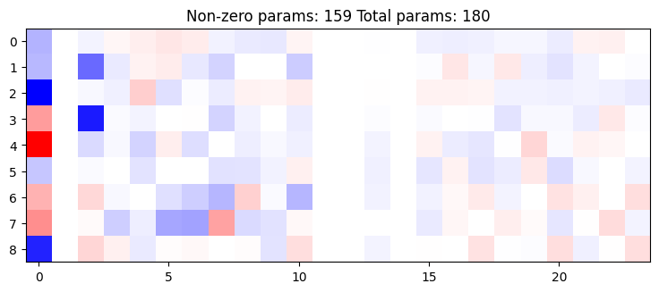
Here the neural net is read as if the representation is written as a vertical vector placed to the right of the image. The vector is then multiplied by the weight matrix to the left of the column, followed by the bias vector to the left of the weight matrix. Not shown is the ReLU activation function (represented by the larger gap), and then the next layer of computation.
The funny part is that 159 floating point numbers is still way too much to memorize. We can begin to improve this by using a funny little technique analogous to quantization-aware training: digit-aware training! We can round the forward pass to the nearest single tens digit, but compute the gradient and update weights at full precision, and use the straight-through estimator for the backward pass. This also adds a small variance to the optimization process, but this turns out to not affect much. Gemini wrote this part of the code for me:
1
2
3
4
5
6
7
8
9
10
11
12
13
14
15
16
17
18
19
20
21
22
23
24
25
# NOTE this code was written by Gemini
class RoundToInt(torch.autograd.Function):
    @staticmethod
    def forward(ctx, weight, scale=1.0):
        # Scale weights so they span across integer steps, then round
        scaled_weight = weight * scale
        rounded_weight = torch.round(scaled_weight)
        # Scale back down for the forward pass (or keep unscaled depending on your architecture)
        return rounded_weight / scale

    @staticmethod
    def backward(ctx, grad_output):
        # Straight-Through Estimator: pass gradients straight through unmodified
        return grad_output, None

class IntegerWeightLinear(nn.Linear):
    def __init__(self, in_features, out_features, bias=True, scale=10.0):
        super().__init__(in_features, out_features, bias)
        self.scale = scale  # Controls the resolution/range of your integer weights

    def forward(self, input):
        # Quantize weights for the forward pass
        w_quantized = RoundToInt.apply(self.weight, self.scale)
        b_quantized = RoundToInt.apply(self.bias, self.scale)
        return F.linear(input, w_quantized, b_quantized)
What is so cool with digit aware training on a ReLU only network is that we can scale the weights easily and keep the final behavior, as $\text{ReLU}(cx) = c\text{ReLU}(x)$ for scalar $c$. If we write our network as
and all parameters $W_1, b_1, W_2, b_2$ have one significant decimal digit, then we can scale all weights by $c=10$
\[\text{ReLU}(cW_1 x) + cb_1 = c\text{ReLU}(W_1 x) + cb_1 = ch\] \[cW_2 ch + c^2 b_2 = c^2o.\]As the decision is simply an argmax function, scaling preserves the decision boundary for all data points while having only integer parameters! We could repeat this process on the full network, but there is more we can do to cut the parameter count down.
Two Simple Neural Position Classifiers
One might hope that one could construct derived features to construct a linear discriminator. However no combination of pairs or triplets of products of elements of the representations of the 638 positions linearly separate the data.
Luckily for us, there are two interesting facts about tic tac toe that can help reduce the amount of numbers to memorize. First, the decision to play in a corner or edge is symmetric up to rotations and reflections. The second is that, just like ImageNet is disproportionately dogs, this dataset is disproportionately playing in the center. We can take advantage of this! The main idea is to create two much smaller learned classifers that will output only if it is optimal to play in the top-left center, and another for the top edge. If other corner or edge positions are legal, the position can simply be rotated to classify that position. And finally if none of these classifiers output that a move there is optimal, and if the center is open then we default to playing in the center. If none of the classifiers output that a move is optimal, and the center is occupied, then we define it such that any legal move is optimal. The pseudo code for this decision function is:
- let $x$ be the $(9,1)$ shape vector of the board, with ‘X’ $\to 1$, ‘O’ $\to -1$, and empty spaces $\to 0$
- let $\text{cornr}(x)$ be the classifier for the top left corner, outputing
Trueif its optimal to play in the top left corner andFalseelse - let $\text{edge}(x)$ be the classifier for the top edge, outputing
Trueif its optimal to play in the top left corner andFalseelse - let $\text{rotate}(x)$ be the clockwise rotation function of the board $x$
- let $\text{decision}(x)$ being defined as:
1
2
3
4
5
6
7
8
9
10
11
12
13
14
15
16
17
18
19
20
21
22
23
24
let optimal_cornr_found = False
for _ in range(4):
  # if corner is legal
  if x[0] == 0:
    optimal_cornr_found = cornr(x)
    if optimal_cornr_found:
      return, play that corner
    x = rotate(x)

let optimal_edge_found = False
for _ in range(4):
  # if edge is legal
  if x[1] == 0:
    optimal_edge_found = edge(x)
    if optimal_edge_found:
      return, play that corner
    x = rotate(x)

if not optimal_cornr_found and not optimal_edge_found:
  # if corner is legal
  if x[4] == 0:
    return, play the center
  else:
    return, play random legal move, guaranteed optimal
This decision function swaps possibly more computation for smaller neural networks, requiring less memorization. This also affects the data we train on.
The Data
Of the 638 non trivial positions, we only need to train $\text{cornr}(x)$ and $\text{edge}(x)$ on certain datapoints knowing that we will use $\text{decision}(x)$ for the final decision. Which data points?
For $\text{cornr}(x)$, we start positions in which the corner is legal to play in. We can remove positions in which the center is optimal, as this is part of the catch all aspect of the decision function. We can remove positions in which every legal move is optimal. This is another aspect of the decision function, in which either the center is legal (and then played), or the center is not legal, and so we know that any move is optimal.
The same applies for $\text{edge}(x)$. This leaves 232 positions to train $\text{cornr}(x)$ on, 187 positions to train $\text{edge}(x)$, and 15 positions in which either the top left corner or the top edge is optimal, but not all moves. Determining which of the 15 should train each classifier is fairly simple. Empirical training runs show that $\text{edge}(x)$ can be done with much less neurons. We therefore train $\text{edge}(x)$ on the 187 positions, and see which of the 15 “either” positions are already classified by the trained $\text{edge}(x)$. This turns out to be 5 of the positions, and so the remaining 10 positions are added to the $\text{cornr}(x)$ dataset.
The Classifers
Training on these datasets gives the following definitions:
\[\begin{eqnarray*} \text{cornr}(x) & : & \\ W_1 & = & \begin{pmatrix} -51 & -32 & -30 & 0 & -20 & -21 & -29 & 0 & 17 \\ -45 & 43 & -20 & -24 & -0 & 54 & -12 & 36 & -14 \\ -36 & -24 & 33 & -27 & -24 & 67 & 0 & -12 & -14 \\ 41 & -28 & -39 & 0 & -16 & 0 & 32 & -39 & -40 \\ 29 & 58 & -21 & -31 & 19 & -22 & -17 & 0 & -18 \\ -28 & -25 & 39 & 0 & 15 & -38 & -25 & -51 & -41 \\ \end{pmatrix}\\ b_1 & = & \begin{pmatrix} 9 \\ 19 \\ 20 \\ -27 \\ 7 \\ -15 \end{pmatrix}\\ W_2 & = & \begin{pmatrix} 66 & -84 & 55 & -100 & 49 & -88 \end{pmatrix} \\ b_2 & = & \begin{pmatrix} -300 \end{pmatrix} \\ x & = & \begin{pmatrix} x[1] \\ x[2] \\ x[3] \\ x[4] \\ x[5] \\ x[6] \\ x[7] \\ x[8] \\ x[5]x[7] \end{pmatrix} \\ \text{return} & & W_2 \text{ReLU}(W_1 x + b_1) + b_2 > 0 \end{eqnarray*}\]Notice that in both definitions we redefine $x$ to remove the redundant column,
\[\begin{eqnarray*} \text{edge}(x) & : & \\ W_1 & = & \begin{pmatrix} -20 & -33 & -39 & 0 & -36 & 0 & 33 & 6 & 42 \\ 0 & -34 & -46 & 40 & -64 & -54 & 0 & -35 & 27 \\ 28 & 15 & 18 & 44 & 0 & -20 & -18 & -16 & -36 \\ \end{pmatrix}\\ b_1 & = & \begin{pmatrix} 17 \\ 0 \\ 32 \end{pmatrix}\\ W_2 & = & \begin{pmatrix} -84 & 96 & -67 \end{pmatrix} \\ b_2 & = & \begin{pmatrix} 590 \end{pmatrix} \\ x & = & \begin{pmatrix} x[0] \\ x[2] \\ x[3] \\ x[4] \\ x[5] \\ x[6] \\ x[7] \\ x[8] \\ x[0]x[5] \end{pmatrix} \\ \text{return} & & W_2 \text{ReLU}(W_1 x + b_1) + b_2 > 0 \end{eqnarray*}\]These two classifers total to 87 non zero parameters to memorize, and 101 parameters in total, an almost 50% decrease in parameters from the “naive” neural network solution.
These results give the final low-parameter strategy:
The Strategy
- If there is only one legal move, play it.
- Win: If the player can win, play that move.
- Block: If the opponent will win next move, block that move by playing it..
- Reading left to right from the top row to the bottom row, represent the board with ‘X’ $\to 1$, ‘O’ $\to -1$, and empty spaces $\to 0$, writting each number in a
(9,1)shaped vector called $x$. For example, for this board:
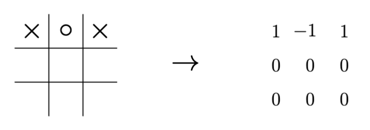
$x = [1, -1, 1, 0, 0, 0, 0, 0, 0]^T$. Then play the move output by $\text{decision}(x)$, defined above.
Further Questions
Can you improve on my result?